import sys
import pandas as pd
import matplotlib
import matplotlib.pyplot as plt
import numpy as np
sys.path.insert(0, "../../")
import spycone as spy
import subprocess
from gtfparse import read_gtf

Transcript-level workflow

Prepare the dataset

The dataset is SARS-Cov-2 infection with 8 time points and 4 replicates.

#sample data
subprocess.call("wget https://zenodo.org/record/7228475/files/tutorial_alt_sorted_bc_tpm.csv?download=1 -O alt_sorted_bc_tpm.csv", shell=True)
subprocess.call("wget https://zenodo.org/record/7228475/files/tutorial_alt_genelist.csv?download=1 -O alt_genelist.csv", shell=True)

data = pd.read_csv("alt_sorted_bc_tpm.csv", sep="\t")
genelist = pd.read_csv("alt_genelist.csv", sep="\t")

geneid= list(map(lambda x: str(int(x)) if not np.isnan(x) else x,  genelist['gene'].tolist()))
transcriptid = genelist['isoforms'].to_list()

Read the data to the dataset function.

dset = spy.dataset(ts=data,
        transcript_id=transcriptid,
        gene_id = geneid,
        species=9606,
        keytype='entrezgeneid',
        timepts=4, reps1=3)

Import biological network of your choice with BioNetwork, Spycone provides Biogrid, IID network in entrez ID as node name. Please specify the keytype if you are using a different ID.

bionet = spy.BioNetwork(path="human", data=(('weight',float),))

Preprocessing

Filtering out genes that has expression across all time points lower than 1. By giving the biological network, it removes genes from the dataset that are not in the network.

spy.preprocess(dset, bionet, cutoff=1)

Detect isoform switch

iso object contains method for isoform switch detect and total isoform usage calculation.

iso = spy.iso_function(dset)
        #run isoform switch
ascov=iso.detect_isoform_switch(filtering=False, min_diff=0.05, corr_cutoff=0.5, event_im_cutoff=0.1, p_val_cutoff=0.05)

iso.detect_isoform_switch returns a dataframe containing the metrics of all isoform switch events detected.

iso_ratio : ratio of switching time to number of time points

diff : difference of relative abundances before and after switch

p_value : combined p-value of maj_pval and min_pval (corresponding p-value from t-test of the transcripts)

corr : dissimilar correlation (inverted pearson correlation)

final_sp : best switch point

event_importance : the ratio of the relative abundance of the events to the highest expressed transcripts

exclusive_domains : domain loss/gain of the event

adj_pval : p-values after multiple test correction

ascov.head()

	gene	gene_symb	major_transcript	minor_transcript	switch_prob	corr	diff	event_importance	exclusive_domains	p_value	adj_pval
0	1019	CDK4	ENST00000552862.1	ENST00000257904.11	1.0	0.822139	0.066160	0.343667	[]	0.002980	0.002838
1	54882	ANKHD1	ENST00000433049.5	ENST00000394722.7	1.0	0.706529	0.073003	0.891058	[PF12796, PF00013]	0.056052	0.039891
2	9140	ATG12	ENST00000379594.7	ENST00000509910.2	1.0	0.613932	0.050557	0.537392	[PF04110]	0.028167	0.022642
3	64419	MTMR14	ENST00000353332.9	ENST00000431250.1	1.0	0.663200	0.062577	0.564498	[]	0.001605	0.001549
4	51184	GPN3	ENST00000228827.8	ENST00000537466.6	1.0	0.913216	0.089762	0.189560	[]	0.001605	0.001549

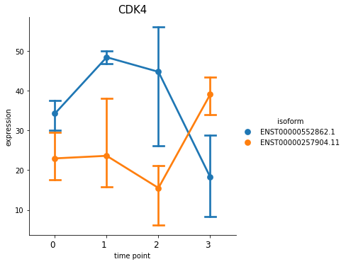
You can also plot out the genes using switch_plot, by provide your dataset object and the result dataframe from detect_isoform_switch.

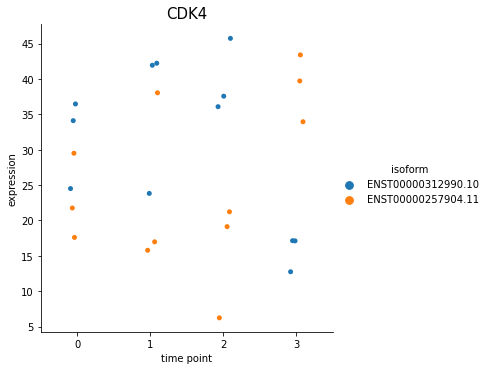
%matplotlib inline
spy.switch_plot("CDK4", dset, ascov)

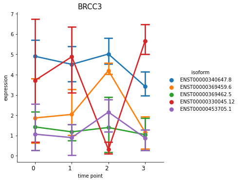
With this function, you can also plot all isoforms in one view, by putting all_isoforms=True.

%matplotlib inline
spy.switch_plot("BRCC3", dset, ascov, all_isoforms=True)

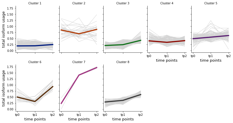
Clustering of total isoform usage

Total isoform usage measures the magnitude of change of isoform relative abundance over time. It indicates the changes due to post-transcriptional regulation (e.g. aternative splicing). You can cluster the genes with total isoform gene, thus getting groups of gene with similar patterns of change of total isoform usage over time.

dset = iso.total_isoform_usage(ascov, gene_level=True)

asclu = spy.clustering(dset, algorithm='hierarchical', metrics="euclidean", linkage="ward", input_type="isoformusage", n_clusters=8, composite=False)
c = asclu.find_clusters()

%matplotlib inline
spy.vis_all_clusters(asclu, col_wrap=5,y_label="total isoform usage")

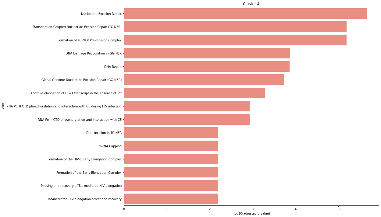
Gene set enrichment analysis

Perform gene set enrichment analysis using clusters_gsea. Change the gene_sets parameter into the choice of your knowledge base or gene set database, e.g. Reactome, KEGG, etc. Use spy.list_genesets to view the available knowledge base.

With the isoform switch detection, we can enriched the domains affect by the isoform switch events using Nease.

Nease only support human at the moment.

asclu_go, _ = spy.clusters_gsea(dset, "hsapiens", is_results=ascov, method="nease", gene_sets = ['Reactome'])

%matplotlib inline
spy.gsea_plot(asclu_go, cluster=4, nterms=15)

DOMINO on the domain level

mods = spy.run_domino(asclu, network_file=bionet, output_file_path="newslices.txt")

Splicing Factor analysis

Perform co-expression analysis to look for splicing factors with similar expression patterns as isoform relative abundance.

sf=spy.SF_coexpression(dset, padj_method="fdr_bh",corr_cutoff=0)
sf_df, cluster_sf = sf.coexpression_with_sf()

Read gtf annotation file for exons information.

# obtain exons gtf, or input customs gtf
subprocess.call("wget https://zenodo.org/record/7229557/files/exons.gtf?download=1 -O exons.gtf", shell=True)
gtf = read_gtf("exons.gtf")

Co-expression analysis result in dataframe sf_df that contains the co-expressed splicing factors and the corresponding cluster. We are specifically interesting in splicing factors that positively and negatively correlated to isoforms in the same gene.

thiscluster=6 #which cluster
end="5p" #specify 3'p or 5'p
sub = sf_df[sf_df['cluster']==thiscluster].drop_duplicates()
subcount = sub.groupby(['iso_genesymb', 'sf']) #extract list of co-expressed splicing factors
subcount = subcount['bin_corr'].agg(sum).reset_index()
subcount=subcount[subcount['bin_corr']==0]

To perform motif search, SF_motifsearch creates a motif object, taking a list of splicing factors, list of genes (e.g. genes in a cluster), dataset object, and the gtf file). Motif searching (search_motifs) will be focusing on loss exons or gain exons with exons parameter and 3p or 5p end with site parameter. Background are the constants exons which can be done by search_background_motifs.

Motif search may take a long time, it is recommended to run in command line environment.

motif=spy.SF_motifsearch(subcount['sf'].unique(), asclu.symbs_clusters[thiscluster], dataset=dset, gtf=gtf)
lossmots = motif.search_motifs(exons="loss", site=end)
gainmots = motif.search_motifs(exons="gain", site=end)
bg = motif.search_background_motifs(site=end)

alldf=motif._df_forvis(lossmots, gainmots, bg=bg)
pvals = motif._get_pvals(alldf)

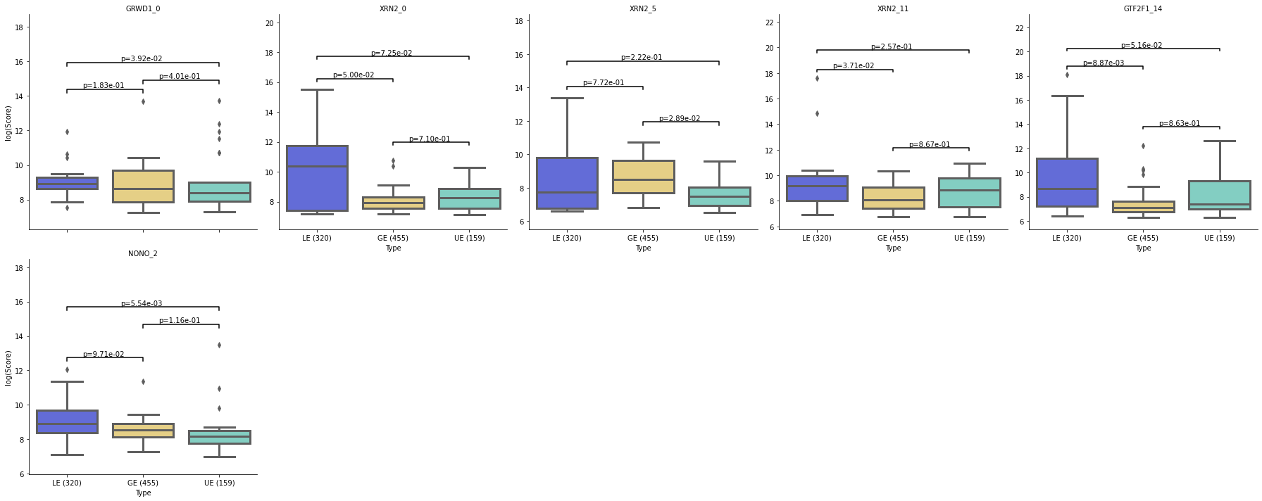
palette = {"lost exons":"#505BEA",
            "gained exons": "#F5D776",
           "background":"#76DACA"}
motif.vis_motif_density(alldf=alldf, pvals=pvals, pval_cutoff=0.05, palette=palette)

<Figure size 576x648 with 0 Axes>